

About This File
This Add-On Instruction Solve the equations System
whit Gauss-Jordan Reduction
In the matrix A [ i , j ] put the System of N-Equation.
In the vector b put the solutions
§§§§§§§§§§§§§§§§§§§§§§§§§§§§§§§§§§§§§§§§§§§§§§§§§
Example 1: Linear System 3 equation (X,Y,Z)
3 X + 2 Y - Z = 10
- X + Y + Z = -2
2 X - Y + 2 Z = -6
| 3 | | 2 | | -1 | | 10 |
X | -1 | + Y | 1 | + Z | 1 | = | -2 |
| 2 | | -1 | | 2 | | -6 |
Matrix A :=
Matrix[1,1]= 3 ; Matrix[1,2]= 2 ; Matrix[1,3]= -1
Matrix[2,1]= -1 ; Matrix[2,2]= 1 ; Matrix[2,3]= -2
Matrix[3,1]= 2 ; Matrix[3,2]= -1 ; Matrix[3,3]= -6
Vector b:=
Vector[1] =10 ; Vector[2] = -2 ; Vector[3] = -6 ;
Solution :=
Solution [1] := 1.0 ; Solution [2] := 2.0 ; Solution [3] := -3.0 ;
X = 1 ; Y = 2 ; Z = -3
§§§§§§§§§§§§§§§§§§§§§§§§§§§§§§§§§§§§§§§§§§§§§§§§§§§§§§§§§§§§§§§§§§
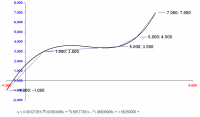
Example 2: Linear System 5 equation for resolve Polynomial 4th grade
exampl. Polynomial whit 5 points:
P0(-1,-1) ;
P1( 1, 3) ;
P2( 5, 3.5) ;
P3( 6, 4.5) ;
P4( 7, 7) ;
Write in the Matrix A [ i, j ]
Matrix A :=
Matrix[1,1]= (-1)^4 ; Matrix[1,2]= (-1)^3 ; Matrix[1,3]= (-1)^2 ; Matrix[1,4]= (-1) ; Matrix[1,5]=1;
Matrix[2,1]= (1)^4 ; Matrix[2,2]= (1)^3 ; Matrix[2,3]= (1)^2 ; Matrix[2,4]= (1) ; Matrix[2,5]=1;
Matrix[3,1]= (5)^4 ; Matrix[3,2]= (5)^3 ; Matrix[3,3]= (5)^2 ; Matrix[3,4]= (5) ; Matrix[3,5]=1;
Matrix[4,1]= (6)^4 ; Matrix[4,2]= (6)^3 ; Matrix[4,3]= (6)^2 ; Matrix[4,4]= (6) ; Matrix[4,5]=1;
Matrix[5,1]= (7)^4 ; Matrix[5,2]= (7)^3 ; Matrix[5,3]= (7)^2 ; Matrix[5,4]= (7) ; Matrix[5,5]=1;
Write in the Vector [ ]
Vector b:=
Vector[1] = -1 ; Vector[2] = 3 ; Vector[3] = 3.5 ; Vector[4] = 4.5 ; Vector[5] = 7
Solutions :=
Solution [1] := 3.27380234e-003 ; Solution [2] := 0.03363105;
Solution [3] := -0.56577414 ; Solution [4] := 1.966369 ;
Solution [5] := 1.5625005
§§§§§§§§§§§§§§§§§§§§§§§§§§§§§§§§§§§§§§§§§§§§§§§§§§§§§§§§§§§§§§§§§§
Example 3: Linear System 6 equation for resolve Polynomial 5th grade
example. Mototion Interpolation whit Polynomial
whit 2 Points :
P0 (Time0, Position 0) Start point whit (Velocity 0, Acceleration 0)
P1 (Time1, Position 1) End point whit (Velocity 1, Acceleration 1)
Write in the Matrix A [ i, j ]
Matrix A :=
X0 = time0 ; X1 = time1
Row1 X0 ^5 + X0 ^4 + X0 ^3 + X0 ^2 + X0 + 1 (Position P0)
Row2 5 * X0 ^4 + 4 * X0 ^3 + 3 * X0 ^2 + 2 * X0 + 1 + 0 (Velocity P0)
Row3 20 * X0 ^3 + 12 * X0 ^2 + 6 * X0 + 2 + 0 + 0 (Acceleration P0)
Row4 X1 ^5 + X1 ^4 + X1 ^3 + X1 ^2 + X1 + 1 (Position P1)
Row5 5 * X1 ^4 + 4 * X1 ^3 + 3 * X1 ^2 + 2 * X1 + 1 + 0 (Velocity P1)
Row6 20 * X1 ^3 + 12 * X1 ^2 + 6 * X1 + 2 + 0 + 0 (Acceleration P1)
Vector b:=
Vector[1] = Position P0 ; Vector[2] = Velocity P0 ; Vector[3] = Acceleration P0 ;
Vector[4] = Position P1 ; Vector[5] = Velocity P1 ; Vector[6] = Acceleration P1 ;
Interpolation Polynomial Position :=
Position := s1* t^5 + s2* t^4 +s3* t^3 + s4* t^2 + s5* t + s6;